15. NumPy vs Numba vs JAX#

15.1.1. Problem Statement#

Consider the problem of maximizing a function $f$ of two variables $(x,y)$ over the square $[-a,a]\times [-a,a]$.

For $f$ and $a$ let’s choose

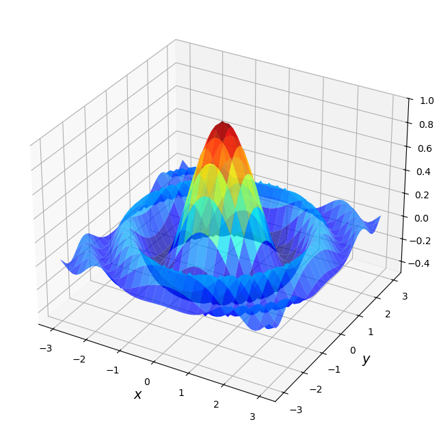
Here’s a plot of $f$

def f(x, y):
    return np.cos(x**2 + y**2) / (1 + x**2 + y**2)

xgrid = np.linspace(-3, 3, 50)
ygrid = xgrid
x, y = np.meshgrid(xgrid, ygrid)

fig = plt.figure(figsize=(10, 8))
ax = fig.add_subplot(111, projection='3d')
ax.plot_surface(x,
                y,
                f(x, y),
                rstride=2, cstride=2,
                cmap=cm.jet,
                alpha=0.7,
                linewidth=0.25)
ax.set_zlim(-0.5, 1.0)
ax.set_xlabel('$x$', fontsize=14)
ax.set_ylabel('$y$', fontsize=14)
plt.show()

For the sake of this exercise, we’re going to use brute force for the maximization.

1. Evaluate $f$ for all $(x,y)$ in a grid on the square.

2. Return the maximum of observed values.

Just to illustrate the idea, here’s a non-vectorized version that uses Python loops.

grid = np.linspace(-3, 3, 50)
m = -np.inf
for x in grid:
    for y in grid:
        z = f(x, y)
        if z > m:
            m = z

15.1.2. NumPy vectorization#

If we switch to NumPy-style vectorization we can use a much larger grid and the code executes relatively quickly.

Here we use np.meshgrid to create two-dimensional input grids x and y such that f(x, y) generates all evaluations on the product grid.

(This strategy dates back to Matlab.)

grid = np.linspace(-3, 3, 3_000)
x, y = np.meshgrid(grid, grid)

with qe.Timer(precision=8):
    z_max_numpy = np.max(f(x, y))

print(f"NumPy result: {z_max_numpy}")

0.25463414 seconds elapsed
NumPy result: 0.9999979986680024

In the vectorized version, all the looping takes place in compiled code.

Moreover, NumPy uses implicit multithreading, so that at least some parallelization occurs.

(The parallelization cannot be highly efficient because the binary is compiled before it sees the size of the arrays x and y.)

15.1.3. A Comparison with Numba#

Now let’s see if we can achieve better performance using Numba with a simple loop.

import numba

@numba.jit
def compute_max_numba(grid):
    m = -np.inf
    for x in grid:
        for y in grid:
            z = np.cos(x**2 + y**2) / (1 + x**2 + y**2)
            if z > m:
                m = z
    return m

grid = np.linspace(-3, 3, 3_000)

with qe.Timer(precision=8):
    compute_max_numba(grid)

0.28494620 seconds elapsed

with qe.Timer(precision=8):
    compute_max_numba(grid)

0.13257146 seconds elapsed

Depending on your machine, the Numba version can be a bit slower or a bit faster than NumPy.

On one hand, NumPy combines efficient arithmetic (like Numba) with some multithreading (unlike this Numba code), which provides an advantage.

On the other hand, the Numba routine uses much less memory, since we are only working with a single one-dimensional grid.

15.1.4. Parallelized Numba#

Now let’s try parallelization with Numba using prange:

Here’s a naive and incorrect attempt.

@numba.jit(parallel=True)
def compute_max_numba_parallel(grid):
    n = len(grid)
    m = -np.inf
    for i in numba.prange(n):
        for j in range(n):
            x = grid[i]
            y = grid[j]
            z = np.cos(x**2 + y**2) / (1 + x**2 + y**2)
            if z > m:
                m = z
    return m

Usually this returns an incorrect result:

z_max_parallel_incorrect = compute_max_numba_parallel(grid)
print(f"Incorrect parallel Numba result: {z_max_parallel_incorrect}")
print(f"NumPy result: {z_max_numpy}")

Incorrect parallel Numba result: -inf
NumPy result: 0.9999979986680024

The incorrect parallel implementation typically returns -inf (the initial value of m) instead of the correct maximum value of approximately 0.9999979986680024.

The reason is that the variable $m$ is shared across threads and not properly controlled.

When multiple threads try to read and write m simultaneously, they interfere with each other, causing a race condition.

This results in lost updates—threads read stale values of m or overwrite each other’s updates—and the variable often never gets updated from its initial value of -inf.

Here’s a more carefully written version.

@numba.jit(parallel=True)
def compute_max_numba_parallel(grid):
    n = len(grid)
    row_maxes = np.empty(n)
    for i in numba.prange(n):
        row_max = -np.inf
        for j in range(n):
            x = grid[i]
            y = grid[j]
            z = np.cos(x**2 + y**2) / (1 + x**2 + y**2)
            if z > row_max:
                row_max = z
        row_maxes[i] = row_max
    return np.max(row_maxes)

Now the code block that for i in numba.prange(n) acts over is independent across i.

Each thread writes to a separate element of the array row_maxes.

Hence the parallelization is safe.

Here’s the timings.

with qe.Timer(precision=8):
    compute_max_numba_parallel(grid)

1.18451452 seconds elapsed

with qe.Timer(precision=8):
    compute_max_numba_parallel(grid)

0.03486371 seconds elapsed

If you have multiple cores, you should see at least some benefits from parallelization here.

For more powerful machines and larger grid sizes, parallelization can generate major speed gains, even on the CPU.

15.1.5. Vectorized code with JAX#

In most ways, vectorization is the same in JAX as it is in NumPy.

But there are also some differences, which we highlight here.

Let’s start with the function.

@jax.jit
def f(x, y):
    return jnp.cos(x**2 + y**2) / (1 + x**2 + y**2)

As with NumPy, to get the right shape and the correct nested for loop calculation, we can use a meshgrid operation designed for this purpose:

grid = jnp.linspace(-3, 3, 3_000)
x_mesh, y_mesh = np.meshgrid(grid, grid)

with qe.Timer(precision=8):
    z_max = jnp.max(f(x_mesh, y_mesh)).block_until_ready()

W1128 00:32:50.770457    2510 cuda_executor.cc:1802] GPU interconnect information not available: INTERNAL: NVML doesn't support extracting fabric info or NVLink is not used by the device.
W1128 00:32:50.773907    2440 cuda_executor.cc:1802] GPU interconnect information not available: INTERNAL: NVML doesn't support extracting fabric info or NVLink is not used by the device.

0.36362576 seconds elapsed

Let’s run again to eliminate compile time.

with qe.Timer(precision=8):
    z_max = jnp.max(f(x_mesh, y_mesh)).block_until_ready()

0.01939678 seconds elapsed

Once compiled, JAX is significantly faster than NumPy due to GPU acceleration.

The compilation overhead is a one-time cost that pays off when the function is called repeatedly.

15.1.6. JAX plus vmap#

There is one problem with both the NumPy code and the JAX code:

While the flat arrays are low-memory

grid.nbytes 

12000

the mesh grids are memory intensive

x_mesh.nbytes + y_mesh.nbytes

72000000

This extra memory usage can be a big problem in actual research calculations.

Fortunately, JAX admits a different approach using jax.vmap.

# Set up f to compute f(x, y) at every x for any given y
f_vec_x = lambda y: f(grid, y)
# Create a second function that vectorizes this operation over all y
f_vec = jax.vmap(f_vec_x)

with qe.Timer(precision=8):
    z_max = jnp.max(f_vec(grid))
    z_max.block_until_ready()

0.10907602 seconds elapsed

with qe.Timer(precision=8):
    z_max = jnp.max(f_vec(grid))
    z_max.block_until_ready()

0.00109720 seconds elapsed

15.1.7. vmap version 2#

We can be still more memory efficient using vmap.

While we avoid large input arrays in the preceding version, we still create the large output array f(x,y) before we compute the max.

Let’s try a slightly different approach that takes the max to the inside.

Because of this change, we never compute the two-dimensional array f(x,y).

@jax.jit
def compute_max_vmap_v2(grid):
    # Construct a function that takes the max along each row
    f_vec_x_max = lambda y: jnp.max(f(grid, y))
    # Vectorize the function so we can call on all rows simultaneously
    f_vec_max = jax.vmap(f_vec_x_max)
    # Call the vectorized function and take the max
    return jnp.max(f_vec_max(grid))

Here

• f_vec_x_max computes the max along any given row

• f_vec_max is a vectorized version that can compute the max of all rows in parallel.

We apply this function to all rows and then take the max of the row maxes.

Let’s try it.

with qe.Timer(precision=8):
    z_max = compute_max_vmap_v2(grid).block_until_ready()

0.24891353 seconds elapsed

Let’s run it again to eliminate compilation time:

with qe.Timer(precision=8):
    z_max = compute_max_vmap_v2(grid).block_until_ready()

0.00040984 seconds elapsed

If you are running this on a GPU, as we are, you should see another nontrivial speed gain.

15.1.8. Summary#

In our view, JAX is the winner for vectorized operations.

It dominates NumPy both in terms of speed (via JIT-compilation and parallelization) and memory efficiency (via vmap).

Moreover, the vmap approach can sometimes lead to significantly clearer code.

While Numba is impressive, the beauty of JAX is that, with fully vectorized operations, we can run exactly the same code on machines with hardware accelerators and reap all the benefits without extra effort.

Moreover, JAX already knows how to effectively parallelize many common array operations, which is key to fast execution.

For almost all cases encountered in economics, econometrics, and finance, it is far better to hand over to the JAX compiler for efficient parallelization than to try to hand code these routines ourselves.

15.2.1. Numba Version#

Here’s the Numba version.

@numba.jit
def qm(x0, n, α=4.0):
    x = np.empty(n+1)
    x[0] = x0
    for t in range(n):
      x[t+1] = α * x[t] * (1 - x[t])
    return x

Let’s generate a time series of length 10,000,000 and time the execution:

n = 10_000_000

with qe.Timer(precision=8):
    x = qm(0.1, n)

0.16079402 seconds elapsed

Let’s run it again to eliminate compilation time:

with qe.Timer(precision=8):
    x = qm(0.1, n)

0.07165647 seconds elapsed

Numba handles this sequential operation very efficiently.

Notice that the second run is significantly faster after JIT compilation completes.

Numba’s compilation is typically quite fast, and the resulting code performance is excellent for sequential operations like this one.

15.2.2. JAX Version#

Now let’s create a JAX version using lax.scan:

(We’ll hold n static because it affects array size and hence JAX wants to specialize on its value in the compiled code.)

from jax import lax
from functools import partial

cpu = jax.devices("cpu")[0]

@partial(jax.jit, static_argnums=(1,), device=cpu)
def qm_jax(x0, n, α=4.0):
    def update(x, t):
        x_new = α * x * (1 - x)
        return x_new, x_new

    _, x = lax.scan(update, x0, jnp.arange(n))
    return jnp.concatenate([jnp.array([x0]), x])

This code is not easy to read but, in essence, lax.scan repeatedly calls update and accumulates the returns x_new into an array.

Let’s time it with the same parameters:

with qe.Timer(precision=8):
    x_jax = qm_jax(0.1, n).block_until_ready()

0.12644219 seconds elapsed

Let’s run it again to eliminate compilation overhead:

with qe.Timer(precision=8):
    x_jax = qm_jax(0.1, n).block_until_ready()

0.06671596 seconds elapsed

JAX is also efficient for this sequential operation.

Both JAX and Numba deliver strong performance after compilation, with Numba typically (but not always) offering slightly better speeds on purely sequential operations.

15.2.3. Summary#

While both Numba and JAX deliver strong performance for sequential operations, there are significant differences in code readability and ease of use.

The Numba version is straightforward and natural to read: we simply allocate an array and fill it element by element using a standard Python loop.

This is exactly how most programmers think about the algorithm.

The JAX version, on the other hand, requires using lax.scan, which is significantly less intuitive.

Additionally, JAX’s immutable arrays mean we cannot simply update array elements in place, making it hard to directly replicate the algorithm used by Numba.

For this type of sequential operation, Numba is the clear winner in terms of code clarity and ease of implementation, as well as high performance.